March Madness At-Large Projector
HomeRepository
Check out the full code and data on GitHub.
Overview
The NCAA College Basketball Tournament, better known as March Madness, is a 68-team, single elimination tournament held every spring to determine the national champion. The selection process for the tournament is complex, with 31 teams receiving automatic bids by winning their respective conference tournaments, and 37 teams receiving at-large bids based on their performance during the regular season and conference tournaments. This project aims to predict which teams will receive at-large bids using machine learning techniques, leveraging historical data and team metrics from the 2019 to 2025 seasons. Also, this project will provide insights into the factors that influence at-large selections, by looking at metrics like SOR (Strength of Record), NET (NCAA Evaluation Tool), number of Quad 1 wins and Quad 3 and 4 losses, and KenPom ratings.
The model achieved 96% accuracy in predicting which teams would receive at-large bids, especially in the 2025 season, where the model predicted 36 of the 37 at-large teams, outperforming expert analyst such as ESPN's Joe Lunardi and CBS Sports' Jerry Palm.
Tech Stack
- R (tidyverse, rvest, stringr)
- Microsoft Excel
- ggplot2 for data visualizations
- Git/GitHub
Data Sources
- Bart Torvik's T-Rank - Team Metrics and Seeding
- College Basketball Reference - Conference Tournament Winners
Project Highlights
- 🧠 Obtained data using web-scraping (rvest) from data sources.
- 📈 Cleaned and formatted data to obtain team metric and seed data for every team. Fixed descrepancies between the two data sources.
- 🏀 Created a logistic model and obtained model diagnostics
- 📊 Visualized EDA findings and model confusion tabel
Exploratory Data Analysis
Before building the model, I performed exploratory data analysis (EDA) to understand the data and identify the mean and median values for the five metrics I am focusing on for teams that received an at-large bid.
| Metric | Mean | Median |
|---|---|---|
| NET | 29.45 | 27 |
| KenPom | 28.99 | 26 |
| SOR | 27.58 | 26 |
| Q1 Wins | 5.73 | 5 |
| Q3 + Q4 Losses | 0.8 | 0 |
From our initial findings, teams that receive an at-large bid have an average NET, KenPom, and SOR of about 28. This isn't a cutoff, just an average of all of those teams. Additionally, teams typically have at least 5 Q1 wins and no more than 1 Q3 or Q4 loss, which demonstrates the importance of quality wins and avoiding even two bad losses in the selection process.
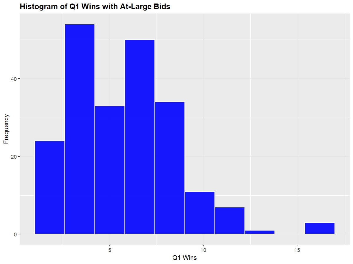
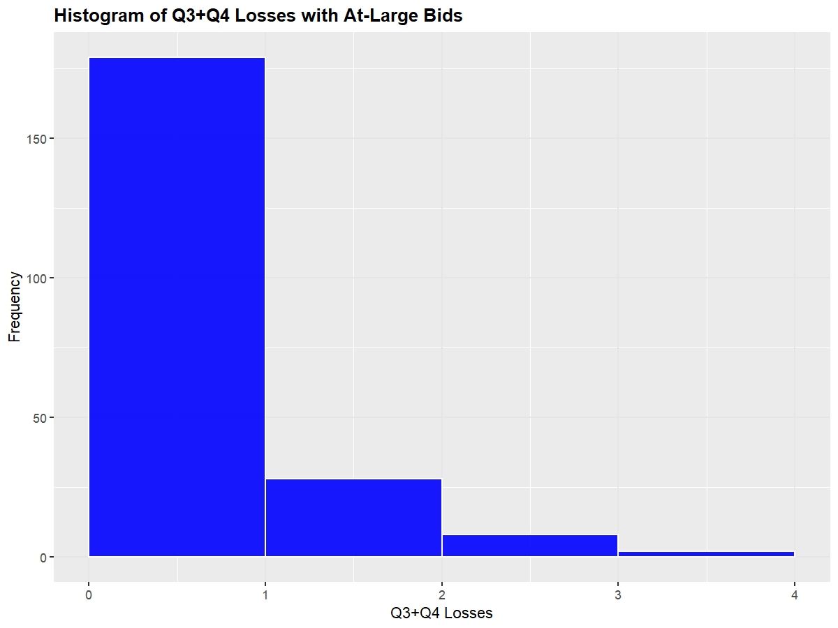
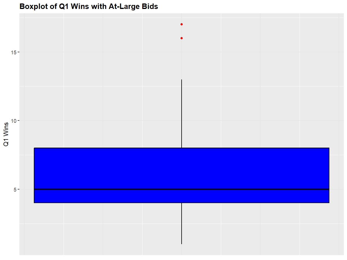
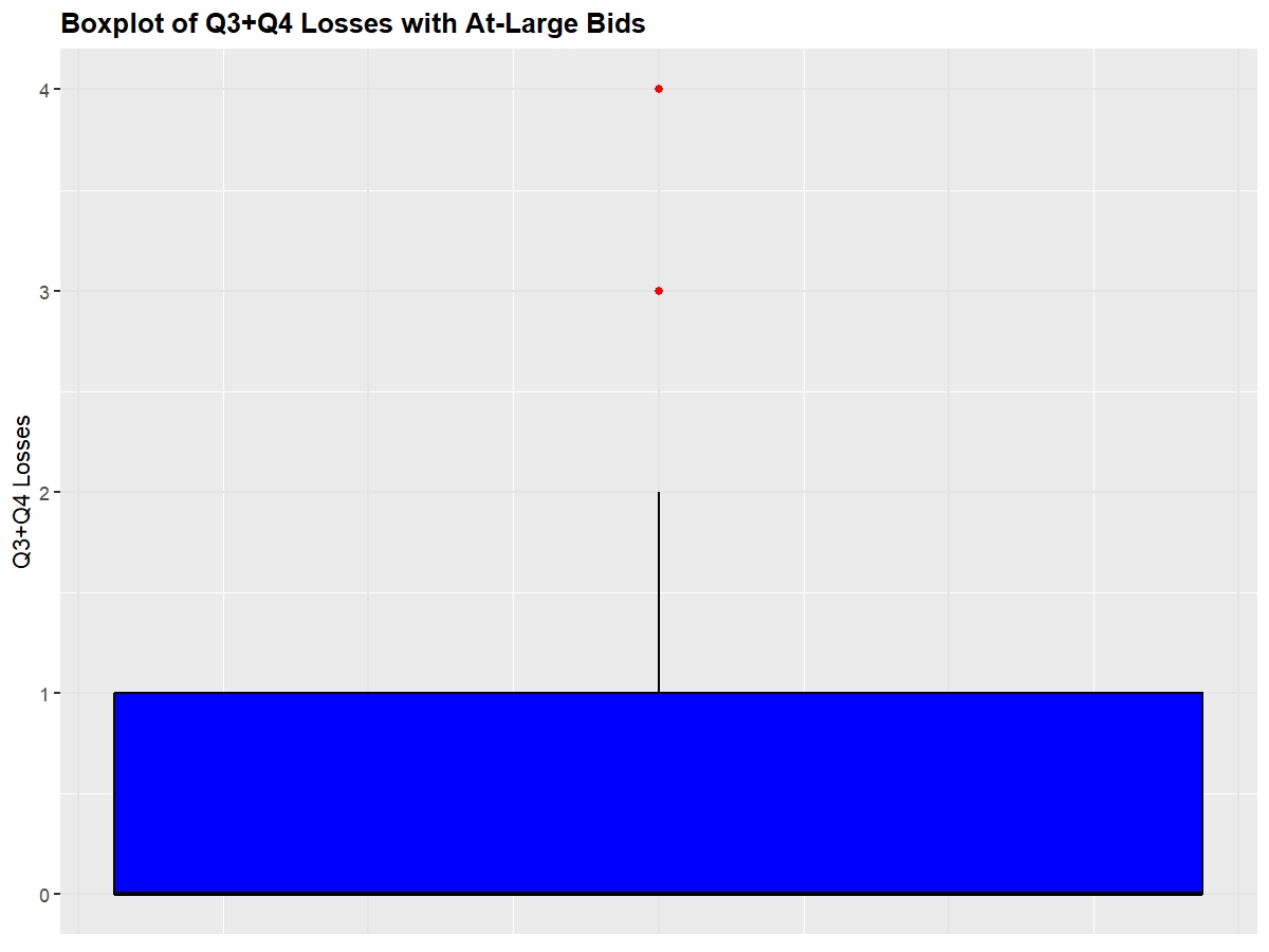
Shown below are the distributions of at-large team's NET, Q1 Wins, and Q3+Q4 Losses (I omitted SOR and KenPom because they're essentially equivalent to NET)
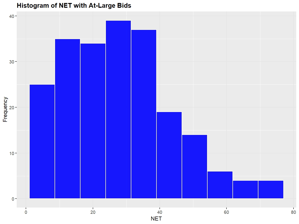
As expected with count data, the distribution is right skewed, with the mean sitting at about 29. The team with the highest (worse) NET to receive an at-large bid was the 2022 Rutgers at 77.
Next, we'll look at a boxplot of these same metrics to observe each of the quantile ranges so that we can observe where teams have to be around so that they feel safe going into Selection Sunday.
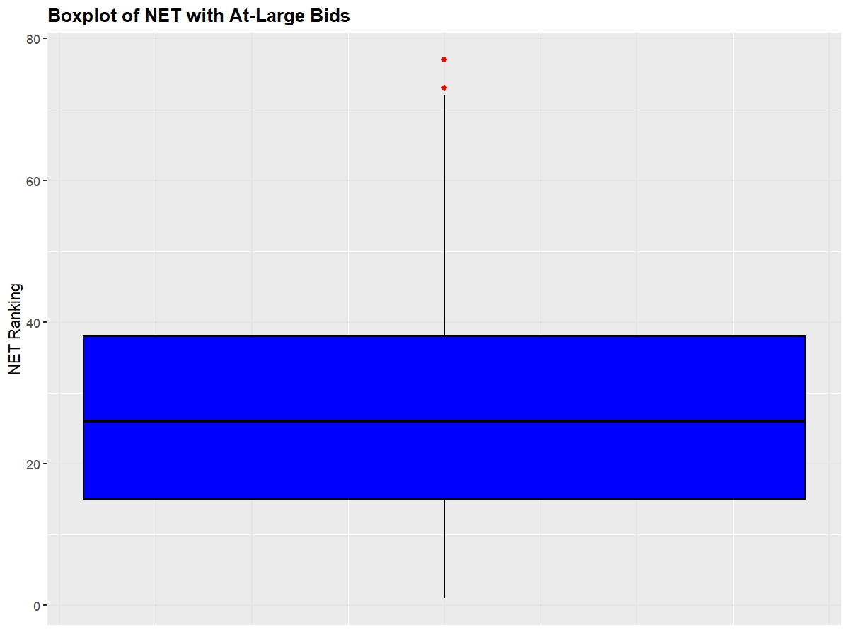
25 Percentile: 15, 75 Percentile: 38
Full Logistic Regression Model
First, I built the Logistic Regression model using all five variables. As always, I split the data into training and testing data
| Variable | Estimate | Std. Error | z value | Pr(>|z|) | Significance |
|---|---|---|---|---|---|
| (Intercept) | -35.9852 | 5.4925 | -6.552 | 5.69e-11 | *** |
| NET | -3.6680 | 1.8226 | -2.012 | 0.04417 | * |
| SOR | -13.9120 | 3.0379 | -4.580 | 4.66e-06 | *** |
| KenPom | -9.2484 | 2.3500 | -3.936 | 8.30e-05 | *** |
| Q1 Wins | 0.9786 | 0.3335 | 2.934 | 0.00335 | ** |
| Q3+Q4 Losses | 1.6635 | 1.4631 | 1.137 | 0.25556 |
Looking at the model output, all but variable Q3+Q4 losses were deemed significant with a p-value < 0.05 with reasonable coefficients for each of the variables (having a higher NET would decrease your log odds, etc.) However, having a positive coefficient for Q3+Q4 Losses which is counterintuitive. My first hunch would be due to multicollinearity, however, checking the VIF values for the model, each variable sits near 1, indicating no multicollinearity issues. Or, teams that had a high number of Q3+Q4 losses made that up by having great metrics, so the model thinks that there is no issue in having a high number of bad losses. Later on, I will use LASSO regression to shrink unneccessary variables to zero.
Still, this full model had an impressive pseudo-R squared value of 0.9 and an AIC of 101.
When making predictions onto the testing dataset, I decided to make it where teams with the top 37 probabilities would be given the bid. Also, because not all years are equivalent in the strength of the bubble, I decided to make these predictions based on an adjusted min-max probabilities where the total sum of probabilities for each year would equal 37. This way, the model can be used to predict the bubble for any year.
Confusion Matrix
| Reference \\ Prediction | FALSE | TRUE |
|---|---|---|
| FALSE | 294 | 2 |
| TRUE | 2 | 35 |
This Confusion Table shows that the model was able to successfully identify the correct status of at-large teams 329/333 times for an accuracy rating of 98.8%. However, this percentage is inflated by the model correctly identifying teams that had no buisness making the tournament. The real test of the model is looking at how it predicted teams that made the tournament and actually made the tournament. So, this model was able to correctly identify 35 of the 37 at-large teams for an accuracy of 94.6%.
Repository
Check out the full code and data on GitHub.